Calculating Groundwater
In the preceding notebooks, we have gathered and processed all the required variables to compute groundwater anomalies.
Recall the equation for calculating groundwater anomalies:

Here, ΔTWS represents the terrestrial water storage anomalies that we have acquired and processed from GRACE. ΔSM stands for soil moisture anomalies derived from GLDAS, while ΔSWE signifies snow water equivalent anomalies, also from GLDAS. Finally, ΔSW refers to surface water anomalies obtained from the USGS and the Bureau of Reclamation.
With these data in hand, we are now ready to calculate groundwater anomalies.
# Load the Jupyter notebook that has the processed GRACE and GLADS data
%run "04A-Reading & Processing GRACE and GLDAS.ipynb"
# Load the Jupyter notebook that has the processed surface water data
%run "04B-Reading & Processing Surface Water.ipynb"
# Print out the first few lines of the dataframe
grace_gldas_df.head()
# Print out the first few lines of the dataframe
storage_df.head()
final_df = grace_gldas_df.merge(storage_df, on=["time", "lat", "lon"], how="outer")
final_df['storage_anomaly_km3'] = final_df['storage_anomaly_km3'].fillna(0) #making NaN values 0 for reservoir data
final_df['storage_acrefeet'] = final_df['storage_acrefeet'].fillna(0) #making NaN values 0 for reservoir data
final_df['storage_km3'] = final_df['storage_km3'].fillna(0) #making NaN values 0 for reservoir data

# Select only the necessary columns
final_df = final_df[['time', 'lon', 'lat', 'storage_anomaly_km3', 'lwe_thickness_km3', 'uncertainty_km3', 'SWE_anomaly_km3', 'RM_anomaly_km3']]
final_df = final_df.dropna().reset_index()
final_df
# Estimate groundwater anomolies
final_df['gw_estimate_km3'] = final_df['lwe_thickness_km3'] - (final_df['SWE_anomaly_km3'] + final_df['RM_anomaly_km3'] + final_df['storage_anomaly_km3'])
Now, we can print out the final dataframe and see the groundwater estimate at each pixel at every point in time.
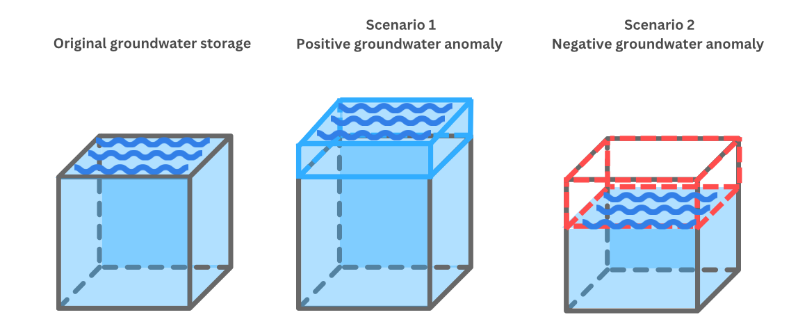
A positive number in the varibale gw_estimate_km3 means that there are more groundwater at the given pixel than the average change in groundwater (the default is 2004-01 to 2009-12 in our code) at the pixel.
A negative number in the varibale gw_estimate_km3 means that there are less groundwater at the given pixel than the average change in groundwater at the pixel.
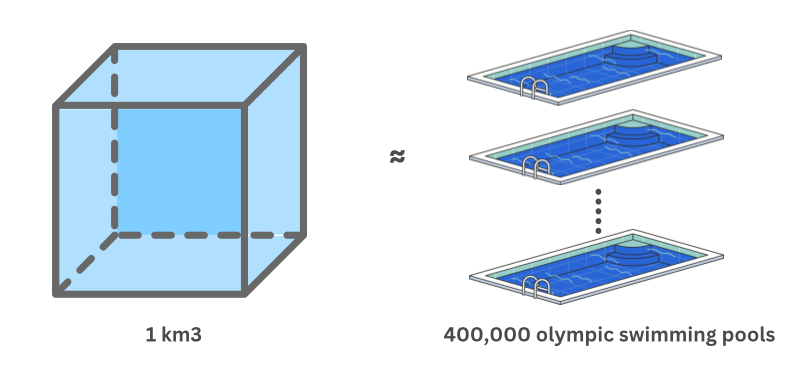
1 kilometer cube of groundwater anomaly is approximately the volume of 400,000 Olympic swimming pools
final_df
Congratulations! You have just constructed a dataset with groundwater anamoly estimates for each pixel in the Colorado River Basin. Below is a time series showing groundwater anomolies in the Basin over time.
# Extracting relevant data from final_df
gw_crb = final_df[['time','gw_estimate_km3']].copy()

# Grouping by 'time' and then computing the mean, followed by resetting the index
gw_crb = gw_crb.groupby(['time']).mean().reset_index()
gw_crb = gw_crb[(gw_crb['time'] >= TIME_PERIOD_START) & (gw_crb['time'] <= TIME_PERIOD_END)]

# Plotting the data
plt.plot('time', 'gw_estimate_km3', data=gw_crb)

# Plotting a horizontal line at y=0
plt.axhline(y=0, color='gray', linestyle='--')  # Here's how you can add the line. Adjust color and linestyle as needed.

# Adding title and labels
plt.title('Groundwater Anomaly Over Time')
plt.xlabel('Time')
plt.ylabel('Groundwater Anomaly (km3)')

# Displaying the plot
plt.show()
Now, we can move on to the next notebook where we can visualize this output in more depth.